Introduction
Here, we provide a breif introduction to linear programming and the simplex algorithm.
Linear Programming
In a linear program, we have a set of decisons we need to make. We represent
each decison as a decison variable. For example,
say we run a small company that sells 2 types of widgets. We must decide how
much of each each widget to produce. Let  and
and  denote the
number of type 1 and type 2 widgets produced respectively.
denote the
number of type 1 and type 2 widgets produced respectively.
Next, we have a set of constraints. Each constraint can be an inequality
( ) or an equality (
 ) but not a strict inequality
(
) but not a strict inequality
( ). Furthermore, it must consist of a linear
combination of the decison variables. For example, let’s say we have a buget of
$20. Type 1 and type 2 widgets cost $2 and $1 to produce respectively. This
gives us our first constraint:
). Furthermore, it must consist of a linear
combination of the decison variables. For example, let’s say we have a buget of
$20. Type 1 and type 2 widgets cost $2 and $1 to produce respectively. This
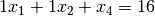
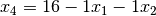
gives us our first constraint: 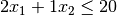 . Furthermore, we can
only store 16 widgets at a time so we can not produce more than 16 total. This
yeilds
. Furthermore, we can
only store 16 widgets at a time so we can not produce more than 16 total. This
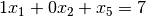
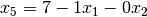
yeilds 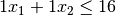 . Lastly, due to enviromental regulations, we
can produce at most 7 type 2 widgets. Hence, our final constraint is
. Lastly, due to enviromental regulations, we
can produce at most 7 type 2 widgets. Hence, our final constraint is
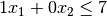 .
.
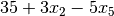
This leaves the final component of a linear program: the objective function.
The objective function specifies what we wish to optimize (either minimize or
maximize). Like constraints, the objective function must be a linear
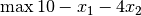
combination of the decison variables. In our example, we wish to maximize
our revenue. Type 1 and type 2 widgets sell for $5 and $3 respectively. Hence,
we wish to maximize  .
.
Combined, the decison variables, constraints, and objective function fully define a linear program. Often, linear programs are written in standard inequality form. Below is our example in standard inequality form.
 |
|
 |
|
|
|
|
|
 |
Let us now summarize the three componets of a linear program in a general sense.
- Decision variables
- The decision variables encode each “decision” that must be made and are
often denoted
 .
.
- Constraints
- The set of constraints limit the values of the decision variables. They
can be inequalities or equalities (
 ) and must consist
of a linear combination of the decision variables. In standard
inequality form, each constraint has the form:
) and must consist
of a linear combination of the decision variables. In standard
inequality form, each constraint has the form:
 .
.
- Objective Function
- The objective function defines what we wish to optimize. It also must be
a linear combination of the decision variables. In standard inequality
form, the objective function has the form:
 .
.
The decison variables and constraints define the feasible region of a
linear program. The feasible region is defined as the set of all possible
decisions that can feasibly be made i.e. each constraint inequality or
equality holds true. In our example, we only have 2 decision variables. Hence,
we can graph the feasible region with on the x-axis and
on the y-axis.
The area shaded blue denotes the feasible region. Any point  in this region denotes a feasible set of decisions. Each point in this region
has some objective value. Consider the point where
in this region denotes a feasible set of decisions. Each point in this region
has some objective value. Consider the point where  and
and
 . This point has an objective value of
 . You can move the objective slider to
see all the points with some objective value. This is called an isoprofit
line. If you slide the slider to 40, you will see that
. You can move the objective slider to
see all the points with some objective value. This is called an isoprofit
line. If you slide the slider to 40, you will see that  lies on
the red isoprofit line.
lies on
the red isoprofit line.
We wish to find the point with the maximum objective value. We can solve
this graphically. We continue to increase the objective value until the
isoprofit line no longer intersects with the feasible region. The point of
intersection right before no point on the isoprofit line is feasible is the
optimal solution! In our example, we push the objective value to 56 before
the isoprofit line no longer intersects the feasible region. The only feasible
point with an objective value of 56 is  . We now know that
 and
and  is an optimal solution with an
optimal value of 56. Hence, we should produce 4 type 1 widgets and 12 type
2 widgets to maximize our revenue!
is an optimal solution with an
optimal value of 56. Hence, we should produce 4 type 1 widgets and 12 type
2 widgets to maximize our revenue!
We now know what a linear program (LP) is and how LPs with 2 decision variables can be solved graphically. In the next section, we will introduce the simplex algorithm which can solve LPs of any size!
The Simplex Algorithm
The simplex algorithm relies on LPs being in dictionary form. An LP in dictionary form has the following properties:
- Every constraint is an equality constraint.
- All constants on the RHS are nonnegative.
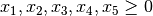
- All variables are restricted to being nonnegative.
- Each variable appears on the left hand side (LHS) or right hand side (RHS). Not both!
- The objective function is in terms of variables on the RHS.
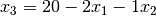
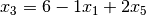
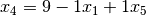
Let us transform our LP example from standard inequality form to dictionary
form. First, we need our constraints to be equalities instead of inequalities.
We have a nice trick for doing this! We can introduce another decision
variable that represents the difference between the linear combination of
variables and the right-hand side (RHS). Hence, the constraint
becomes 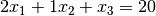 . Note that
this new variable
. Note that
this new variable  must also be nonnegative. After transforming all
of our constraints, we have:
must also be nonnegative. After transforming all
of our constraints, we have:
|
|
|
|
 |
|
 |
|
 |
Recall, we want each variable to appear on only one of the LHS or RHS. We
consider the objective function to be on the RHS. Right now, and
appear on both the LHS and RHS. To fix this, we will move them from
the LHS to the RHS in each constraint. Furthermore, we want the constants on
the RHS so we will do that now as well. This leaves us with:
|
|
|
 |
 |
|
 |
|
|
Our LP is now in dictionary form! This is not the only way to write this LP in
dictionary form. Each dictionary form for an LP has a unqiue dictionary.
The dictionary consists of the variables that only appear on the LHS. The
corresponding dictionary for the above LP is  . Furthermore,
each dictionary has a corresponding feasible solution. This solution is
obtained by setting variables on the RHS to zero. The variables on the LHS
(the variables in the dictionary) are then set to the constants on the RHS.
The corresponding feasible solution for the dictioary is
. Furthermore,
each dictionary has a corresponding feasible solution. This solution is
obtained by setting variables on the RHS to zero. The variables on the LHS
(the variables in the dictionary) are then set to the constants on the RHS.
The corresponding feasible solution for the dictioary is
 or just
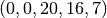 .
.
The driving idea behind the simplex algorithm is that some LPs are easier to
solve that others. For example, the objective function
 is easily maximized by setting
  and
and  . This is because the objective function has only negative
coefficients. Simplex algebraically manipulates an LP (without changing the
objective function or feasible region) in to an LP of this type.
. This is because the objective function has only negative
coefficients. Simplex algebraically manipulates an LP (without changing the
objective function or feasible region) in to an LP of this type.
Let us walk through an iteration of simplex on our example LP. First, we choose
a variable that has a positive coefficent in the objective function. Let us
choose . We call our entering variable. In the
current dictionary, . We want to enter our
dictionary so it can take a positive value and increase the objective
function. To do this, we must choose a constraint where we can solve for
to get on the LHS. Our constraints limit the
increase of so we need to determine the
most limiting constraint. Consider the constraint
. Recall, dictionary form enforces all constants
on the RHS are nonnegative. Hence,  since increasing
by more than 10 would make the constant on the RHS negative. We can
do this for every constraint to get bounds on the increase of .
since increasing
by more than 10 would make the constant on the RHS negative. We can
do this for every constraint to get bounds on the increase of .
|
|
|
 |
|
 |
It follows that the most limiting constraint is .
We now solve for and get
|
|
|
|
|
|
 |
|
|
Now, we must substitute  for everywhere on
the RHS and the objective function so that only appears on the
LHS.
for everywhere on
the RHS and the objective function so that only appears on the
LHS.
|
 |
|
 |
 |
|
 |
|
|
|
 |
|
 |
 |
|
|
|
|
The simplex iteration is now complete! The variable has entered
the dictionary and  has left the dictionary. We call
the leaving variable. Our new dictionary is
has left the dictionary. We call
the leaving variable. Our new dictionary is  and the
corresponding feasible solution is
and the
corresponding feasible solution is
 or just
 . Furthermore, our objective value increased from 0 to 35!
We can continue in this fashion until there is no longer a variable with a positive coefficent in the objective function. We then have an optimal solution. Use the iteration slider below to toggle through iterations of simplex on our example. You can see the updating tableau in the top right and the path of simplex on the plot. Furthermore, you can hover over the corner points to see the feasible solution, dictionary, and objective value at that point.
In summary, in every iteration of simplex, we must
- Choose a variable with a positive coefficient in the objective function.
- Determine how much this variable can increase by finding the most limiting constraint.
- Solve for the entering variable in the most limiting constraint and then substitute on the RHS such that the entering variable no longer appears on the RHS. Hence, it has entered the dictionary!
When there are no positive coefficient in the objective function, we are done!
This concludes our breif introduction to linear programming and the simplex algorithm. In the following tutorial, we will learn how one can use GILP to generate linear programming visualizations like the ones seen in this introduction.
This introduction is based on “Handout 8: Linear Programming and the Simplex Method” from Cornell’s ENGRI 1101 (Fall 2017).