Tutorial
First, open up a Jupyter Notebook or Google Colab enviroment. Reminder: if you
are using a Google Colab enviroment, you will have to reinstall gilp every time
by running the cell !pip install gilp.
Example LPs
GILP comes with many LP examples. Before we use them, we must import them.
from gilp import examples as ex
We can now access the LP examples using ex.NAME where NAME
is the name of the example LP. For example, consider:
 |
 |
 |
 |
 |
|
 |
|
 |
This example LP is called ALL_INTEGER_2D_LP. Let us assign this LP to a
variable called lp.
lp = ex.ALL_INTEGER_2D_LP
Now, we can begin visualizing LPs. We import the visualization function below.
from gilp.visualize import simplex_visual
The function simplex_visual() takes an LP and returns a plotly figure.
The figure can then be viewed on a Jupyter Notebook inline using
simplex_visual(lp).show()
If .show() is run outside a Jupyter Notebook enviroment, the
visualization will open up in the browser. Alternatively, the HTML file can be
written and then opened.
simplex_visual(lp).write_html('name.html')
Here is the resulting visualization from running
simplex_visual(lp).show()
The resulting visualization has the following components.
- Plot:
- On the left, a plot shows the feasible region of the LP shaded in blue. You can hover over the corner points to see the feasible solution, dictionary, and objective value asscociated with that point.
- Constraints:
- In the middle, there is a list of constraints (not including the nonnegativity constraints). You can click on a constraint to mute it and click again to bring it back.
- Dictionary Form LP:
- The dictionary form for the current iteration of simplex is shown in the top right. If the slider is between iterations, the dictionary form for both the previous and next iteration are shown.
- Sliders:
- The iteration slider allows you to toggle through iterations of simplex. You can see the path of simplex on the plot and the updating corresponding dictionary LPs. The objective slider allows you to see the isoprofit line or plane for various objective values.
Defining LPs
We can also create our own LPs! First, we must import the LP class.
from gilp.simplex import LP
The LP class creates linear programs from their standard inequality
form. We can represent a standard inequality form LP in terms of three
matrices.
|
 |
|
 |
 |
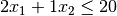
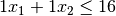
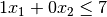
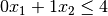
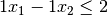
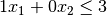
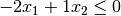
For example, consider the following LP in standard inequality form.
|
 |
|
 |
 |
|
 |
|
 |
|
|
In this example, we have 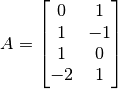 ,
,  , and
, and  . Note

We will use these three matrices to create an instance of LP. First, we
will import NumPy to create the matrices.
import numpy as np
Now, using NumPy, we create the matrices and create the LP instance.
from gilp.simplex import LP
A = np.array([[0, 1],
[1, -1],
[1, 0],
[-2, 1]])
b = np.array([[4],
[2],
[3],
[0]])
c = np.array([[1],
[2]])
# Alternatively
b = np.array([4,2,3,0])
c = np.array([1,2])
lp = LP(A,b,c)
Now, we can visualize it like before!
simplex_visual(lp).show()
The complete code for defining the LP and visualizing it is given below.
1 2 3 4 5 6 7 8 9 10 11 12 13 | import numpy as np from gilp.simplex import LP from gilp.visualize import simplex_visual A = np.array([[0, 1], [1, -1], [1, 0], [-2, 1]]) b = np.array([4,2,3,0]) c = np.array([1,2]) lp = LP(A,b,c) simplex_visual(lp).show() |
Solver Parameters
The simplex_visual() function has some optional solver parameters that
can be set. These include an initial solution, iteration limit, and pivot rule.
We go over each in more detail using ex.KLEE_MINTY_3D_LP as an example.
For reference, here is the visualization of the Klee Minty Cube with no solver
parameters set.
simplex_visual(ex.KLEE_MINTY_3D_LP).show()
Setting an Initial Solution
By default, the intial solution is always set at the origin. However, one can choose from any corner point to be the initial solution. For those with previous experience with LPs, the initial solution must be a basic feasible solution. An initial solution is set as follows:
simplex_visual(lp, initial_solution=x).show()
where x is a NumPy vector representing the initial solution. Above,
you can see the default initial feasible solution is the origin. Let us try
setting a different initial solution.
x = np.array([[0],[25],[25]])
simplex_visual(ex.KLEE_MINTY_3D_LP, initial_solution=x).show()
Iteration Limits
By default, the simplex algorithm will run simplex iterations until an optimal solution is found. Alternatively, an iteration limit can be set:
simplex_visual(lp, iteration_limit=l).show()
where l is an integer iteration limit. Above, you can see it takes 5
simplex iterations to reach the optimal solution. Let’s set the iteration limit
to be 3.
simplex_visual(ex.KLEE_MINTY_3D_LP, iteration_limit=3).show()
Setting a Pivot Rule
Be default, the simplex algorithm uses Bland’s pivot. In addition to Bland’s rule, three other pivot rules are implemented. In an iteration of simplex, the leaving variable is always the minimum (positive) ratio (minimum index to tie break) regardless of the chosen pivot rule. Of the eligible entering variables (those with positive coefficients in the objective function), each pivot rule determines the entering variable as follows:
- Bland’s Rule (reference as
blandormin_index) Minimum index. - Dantzig’s Rule (reference as
dantzigormax_reduced_cost) Most positive reduced cost. - Greatest Ascent (reference as
greatest_ascent) Most positive (minimum ratio) x (reduced cost). - Manual Select (reference as
manual_select) Selected by user.
A desired pivot rule is specified as follows.
simplex_visual(lp, rule=r).show()
where r is a string representing the chosen rule. Let us try some other
pivot rules on ex.KLEE_MINTY_3D_LP!
simplex_visual(ex.KLEE_MINTY_3D_LP, rule='dantzig').show()
simplex_visual(ex.KLEE_MINTY_3D_LP, rule='greatest_ascent').show()
simplex_visual(ex.KLEE_MINTY_3D_LP, rule='manual_select').show()
For this visualization, the chosen entering variables were 2,3, and then 5.
This concludes the quickstart tutorial! See the Development section for information on developing for GILP.